Carburization of a Tube with Fixed Environmental Activity
Purpose: Learn to perform diffusion simulation at constant temperature for a carburization process with an input flux as boundary condition.
Module: PanDiffusion
Thermodynamic and Mobility Database: Fe-Si-C.tdb
Batch file: Example_#4.8.pbfx
Calculation Procedures:
-
Create a workspace and select the PanDiffusion module following Pandat User's Guide: Workspace;
-
Load Fe-Si-C.tdb following the procedure in Pandat User's Guide: Load Database , and select all three components;
-
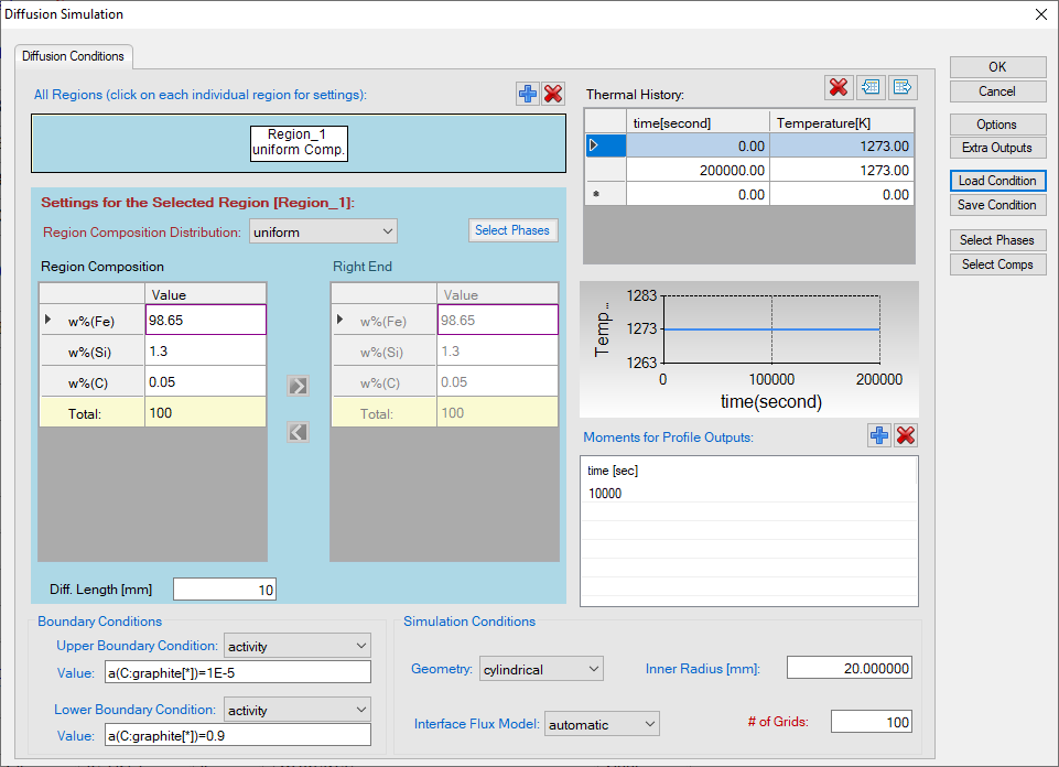
Click on the menu "PanDiffusion → Diffusion Simulation" and set up the calculation condition as shown in Figure 1. First click the red “X” above Regions to delete Region_2 and leave one Region only;
-
Click on Region_1 and set the composition as 0.05C-98.65Fe-1.3Si (wt%), the Diff. Length as 10 mm, and the # of Grids as 200;
-
Click “Select Phase” and set Fcc as the entered phase;
-
The Thermal History is at 1273 K for 2E5 seconds;
-
Click on Upper Boundary Condition and select “activity”, and set the activity value at the right edge of Region_1 as “a(C:graphite[*])=1E-5”. Click on Lower Boundary Condition and select “activity”, then set the activity value at the left edge of Region_1 as “a(C:graphite[*])=0.9”;
-
In order to set a tube geometry, select “cylindrical” in “Geometry”, and apply 20 mm to “Inner Radius”;
-
In the settings shown in Figure 1, composition profiles at the initial and final stages, as well as at 1E4 s, will be outputted. Click OK to perform calculations.
Post Calculation Operation:
-
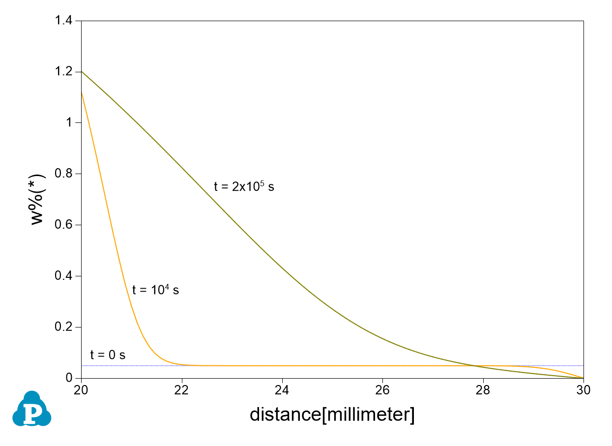
Enlarge the composition range between 0 and 1.4 (wt%) to clearly display Carbon composition. The calculated plot is show in Figure 2Change graph appearance and add text following the procedure in Pandat User's Guide: Property.
Information obtained from this calculation:
-
Learn to set up Boundary conditions for a tube geometry, and fixed activities at both inner and outer surfaces;
-
Observe carbon diffusion from inner surface (high activity) into the tube;